2.4. Model-free estimation of mean age

The mean age of a molecular population equals the area under the labeling survival curve f(t) — the fraction of unlabeled molecules remaining at time t:

\[\bar{\mathcal{A}} = \int_0^\infty f(t)\, dt\]

estimate_mean_age_trapezoid() approximates this integral directly from measured data points, without fitting a parametric compartmental model. This makes it a fast, model-free baseline that can be applied to any labeling experiment.

The function supports two interpolation strategies (controlled by semilogy):

• Linear (semilogy=False): linear interpolation between data points — appropriate when the curve is nearly linear between measurements.

• Log-linear (semilogy=True, the default): exponential interpolation — more accurate for the typical decay shape of labeling curves.

An optional extrapolation step (extrapolate=True, the default) extends the last measured interval to f = 0, capturing the tail area that would otherwise be missed.

from symbolic_compartmental_model import SymbolicCompartmentalModel
import matplotlib.pyplot as plt
import numpy as np
from pathlib import Path

2.4.1. Generating synthetic labeling data

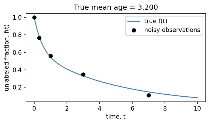
We start by constructing a two-state CM with known parameters so we can compare the trapezoid estimate against the exact analytical mean age.

cm_true = SymbolicCompartmentalModel(n_states=2)
cm_true.contributed_turnovers = [[-0.2, 0.0], [0.0, -2.0]]
cm_true.observed_pool_weights = [0.6, 0.4]

true_mean_age = cm_true.mean_age()
print(f"True mean age: {true_mean_age:.4f}")

rng = np.random.default_rng(seed=42)
tdata = np.array([0.0, 0.3, 1.0, 3.0, 7.0])
ydata_clean = cm_true.f()(tdata)
noise = rng.normal(0, 0.02, size=tdata.shape)
ydata = np.clip(ydata_clean + noise, 1e-6, 1.0)

fig, ax = plt.subplots(1, 1, figsize=(5, 3), dpi=150)
t_fine = np.linspace(0, 10, 300)
ax.plot(t_fine, cm_true.f()(t_fine), color="steelblue", label="true f(t)")
ax.scatter(tdata, ydata, color="black", zorder=5, label="noisy observations")
ax.set_xlabel("time, t")
ax.set_ylabel("unlabeled fraction, f(t)")
ax.legend()
ax.set_title(f"True mean age = {true_mean_age:.3f}")
fig.tight_layout()
if Path("../results").exists():
    fig.savefig("../results/example_trapezoid_data.svg")
display(fig)
plt.close(fig)

True mean age: 3.2000

2.4.2. Applying the trapezoid estimator

Passing an ax argument to estimate_mean_age_trapezoid() produces a diagnostic plot: it draws each interpolation segment as a filled region, making it easy to see exactly how the area is being approximated. The shaded area is the estimated mean age.

fig, ax = plt.subplots(1, 1, figsize=(6, 3.5), dpi=150)

estimated_mean_age = SymbolicCompartmentalModel.estimate_mean_age_trapezoid(
    tdata, ydata, semilogy=True, extrapolate=True, ax=ax
)

ax.set_xlabel("time, t")
ax.set_ylabel("unlabeled fraction, f(t)")
ax.set_title(
    f"Trapezoid estimate = {estimated_mean_age:.3f}   |   True mean age = {true_mean_age:.3f}"
)
fig.tight_layout()
if Path("../results").exists():
    fig.savefig("../results/example_trapezoid_estimate.svg")
display(fig)
plt.close(fig)

print(f"Trapezoid estimate : {estimated_mean_age:.4f}")
print(f"True mean age      : {true_mean_age:.4f}")
print(f"Relative error     : {abs(estimated_mean_age - true_mean_age) / true_mean_age * 100:.1f} %")

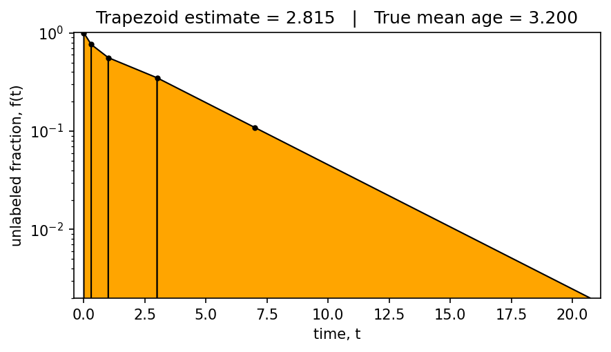
Trapezoid estimate : 2.8147
True mean age      : 3.2000
Relative error     : 12.0 %

The orange shaded regions show the individual trapezoids, with the final segment extrapolated to f = 0 using an exponential tail. The estimate is close to the analytical mean age despite using only 7 noisy data points.

2.4.3. Effect of the extrapolate and semilogy flags

The two optional flags control accuracy:

• ``extrapolate=False``: the integral is truncated at the last observed time point, which systematically underestimates the mean age whenever the curve has not yet reached zero.

• ``semilogy=False``: linear rather than exponential interpolation between consecutive points — less appropriate for the curved shape of typical labeling data but included for comparison.

Here we compare all four combinations on the same dataset.

fig, axs = plt.subplots(2, 2, figsize=(10, 6), dpi=120)

configs = [
    (True,  True,  axs[0, 0]),
    (True,  False, axs[0, 1]),
    (False, True,  axs[1, 0]),
    (False, False, axs[1, 1]),
]

for semilogy, extrapolate, ax in configs:
    est = SymbolicCompartmentalModel.estimate_mean_age_trapezoid(
        tdata, ydata, semilogy=semilogy, extrapolate=extrapolate, ax=ax
    )
    mode = ("log" if semilogy else "linear") + ", " + ("extrap." if extrapolate else "no extrap.")
    error_pct = (est - true_mean_age) / true_mean_age * 100
    ax.set_xlabel("time, t")
    ax.set_ylabel("f(t)")
    ax.set_title(f"{mode}\nestimate = {est:.3f}  (error {error_pct:+.1f} %)")

fig.suptitle(f"True mean age = {true_mean_age:.3f}", fontsize=11)
fig.tight_layout()
if Path("../results").exists():
    fig.savefig("../results/example_trapezoid_flags.svg")
display(fig)
plt.close(fig)

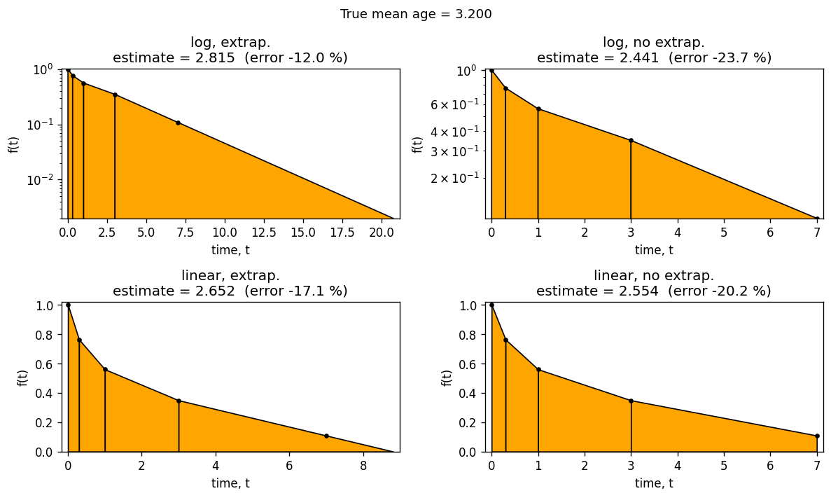
Without extrapolation the estimate is truncated and always underestimates the true mean age. Log-linear interpolation (semilogy=True) is more accurate for exponentially decaying data: it accounts for the curvature between measurement points that linear interpolation misses.

2.4.4. Comparing the trapezoid estimate with model-based estimates

The trapezoid method requires no model assumptions — it only needs the raw (t, f) data. A model-based mean age (obtained by fitting a CM and calling mean_age()) is more accurate when the model is correctly specified, but requires choosing the right model structure. A misspecified model can be worse than the model-free baseline.

Below we fit both a 1-state and a 2-state CM to the same data and compare all three estimates.

cm1 = SymbolicCompartmentalModel(n_states=1)
k = cm1.add_parameter(symbol="k", lb=0.01, ub=10.0)
cm1.contributed_turnovers = [[-k]]
fit1 = cm1.fit(tdata[1:], ydata[1:])

cm2 = SymbolicCompartmentalModel(n_states=2)
k1 = cm2.add_parameter(symbol="k1", lb=0.01, ub=5.0)
k2 = cm2.add_parameter(symbol="k2", lb=0.01, ub=5.0)
w  = cm2.add_parameter(symbol="w",  lb=0.0,  ub=1.0)
cm2.contributed_turnovers = [[-k1, 0.0], [0.0, -k2]]
cm2.observed_pool_weights = [w, 1 - w]
fit2 = cm2.fit(tdata[1:], ydata[1:])

trap_est   = SymbolicCompartmentalModel.estimate_mean_age_trapezoid(tdata, ydata)
age_1state = fit1.cm.mean_age()
age_2state = fit2.cm.mean_age()

print(f"True mean age          : {true_mean_age:.4f}")
print(f"1-state model estimate : {age_1state:.4f}  (error {(age_1state - true_mean_age)/true_mean_age*100:+.1f} %)")
print(f"Trapezoid estimate     : {trap_est:.4f}  (error {(trap_est   - true_mean_age)/true_mean_age*100:+.1f} %)")
print(f"2-state model estimate : {age_2state:.4f}  (error {(age_2state - true_mean_age)/true_mean_age*100:+.1f} %)")

fig, ax = plt.subplots(1, 1, figsize=(6, 3.5), dpi=150)
t_fine = np.linspace(0, 10, 300)
ax.plot(t_fine, cm_true.f()(t_fine), color="steelblue", lw=2,   label=f"true f(t)  (age={true_mean_age:.2f})")
fit1.cm.plot("f", ax=ax, t_range=t_fine, color="tomato",   ls="--", label=f"1-state fit  (age={age_1state:.2f})")
fit2.cm.plot("f", ax=ax, t_range=t_fine, color="seagreen", ls="-.", label=f"2-state fit  (age={age_2state:.2f})")
ax.scatter(tdata, ydata, color="black", zorder=5, s=20, label="data")
ax.set_xlabel("time, t")
ax.set_ylabel("unlabeled fraction, f(t)")
ax.legend(fontsize=8)
ax.set_title(f"Trapezoid estimate = {trap_est:.2f}")
fig.tight_layout()
if Path("../results").exists():
    fig.savefig("../results/example_trapezoid_comparison.svg")
display(fig)
plt.close(fig)

True mean age          : 3.2000
1-state model estimate : 2.2860  (error -28.6 %)
Trapezoid estimate     : 2.8147  (error -12.0 %)
2-state model estimate : 2.9019  (error -9.3 %)

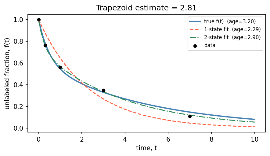
The 1-state model cannot capture the bi-exponential shape, so it is systematically biased and gives the worst mean-age estimate. The trapezoid method, being model-free, does better despite using only a handful of sparse data points. The 2-state model — correctly specified — gives the most accurate estimate, illustrating that a good parametric model outperforms the non-parametric baseline when the model structure is known.

Download notebook

Download this notebook