2.1. Example of model with 2 states

This notebook demonstrates how to construct, visualize, and fit a SymbolicCompartmentalModel (CM) with two internal states.

A compartmental model describes a population of molecules distributed across distinct biochemical states, each with its own turnover rate. The key observable is the labeling curve f(t) — the fraction of unlabeled molecules remaining at time t — which reflects the underlying age distribution of the molecular population.

2.1.1. A simple CM without parameters

We start by creating a two-state CM with fixed (numeric) turnover rates.

• ``n_states``: number of compartments.

• ``contributed_turnovers``: the rate matrix \(\mathbf{M}\). Diagonal entries \(\mathbf{M}[i][i]\) are the (negative) self-turnover rates of each state; off-diagonal entries \(\mathbf{M}[i][j]\) describe the transfer rate from state \(j\) into state \(i\). Here the two states are independent (zero off-diagonals), so state 0 clears at rate 0.5 (half-life ≈ 1.4 time units) and state 1 clears at rate 1.0 (half-life ≈ 0.7 time units).

• ``observed_pool_weights``: the fraction of the total signal contributed by each state (denoted \(\mathbf{s}\), summing up to 1). By default, only the last state contributes to the observed labeling - i.e., \(\mathbf{s} = (0, 0, \ldots, 0, 1)\)

from symbolic_compartmental_model import SymbolicCompartmentalModel
import matplotlib.pyplot as plt
import numpy as np
import scipy
from pathlib import Path
from tqdm.notebook import tqdm

cm1 = SymbolicCompartmentalModel(n_states=2)

cm1.contributed_turnovers = [[-0.5, 0.0], [0.0, -1.0]]

print(cm1.observed_pool_weights)

Matplotlib is building the font cache; this may take a moment.

[0, 1]

fig, ax = plt.subplots(1, 1, figsize=(5, 3), dpi=150)
cm1.plot("f", ax=ax)
fig.tight_layout()
if Path("../results").exists():
    fig.savefig("../results/example_2_state.svg")
plt.close(fig)
display(fig)

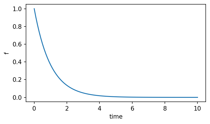
The plot shows f(t) — the survival function of the age distribution, i.e. the probability that a randomly sampled molecule has age greater than t. For a two-state model with independent states this is a weighted sum of two exponential decays. The mean age of the population equals the area under this curve.

2.1.2. Using symbols in CM

2.1.2.1. Parameterizing pool sizes

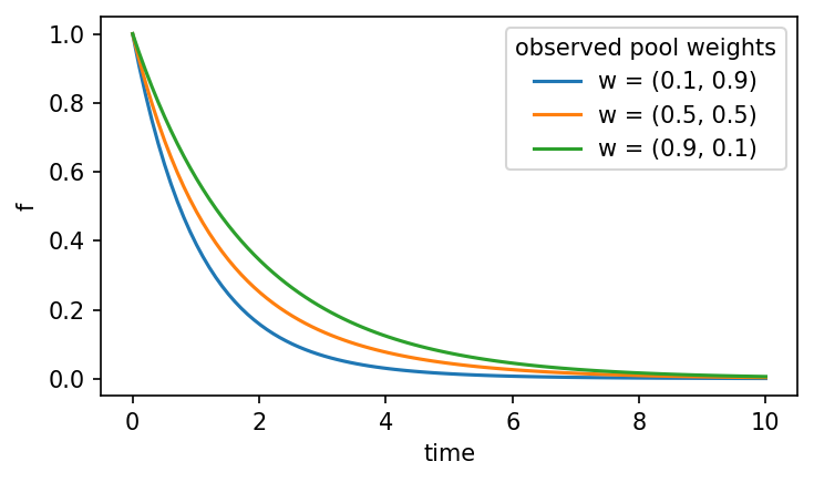
add_parameter() creates a SymPy symbol bound to a named parameter with given bounds. Using a symbolic a for the pool weights means the model represents a family of curves — weight a for state 0 and 1 − a for state 1 — without committing to a specific value yet.

Calling plot() or evaluating any numeric property requires passing concrete values for all free parameters via the x argument.

a = cm1.add_parameter(symbol="a", lb=0.0, ub=1.0)
cm1.observed_pool_weights = [a, 1.0-a]
print(cm1.observed_pool_weights)

[a, 1.0 - a]

try:
    fig, ax = plt.subplots(1, 1, figsize=(5, 3), dpi=150)
    cm1.plot("f", ax=ax)
except AssertionError as e:
    print("AssertionError: " + str(e))

plt.close(fig)

AssertionError: the input must not be empty if the model has at least one parameter

Attempting to plot without supplying a value for a raises an AssertionError, because the model cannot compute f(t) without knowing the pool weights. Passing explicit values via x evaluates the model at each setting and produces one curve per value of a.

fig, ax = plt.subplots(1, 1, figsize=(5, 3), dpi=150)
for a_value in [0.1, 0.5, 0.9]:
    cm1.plot("f", x=[a_value], ax=ax, label=f"w = ({a_value:.1f}, {1-a_value:.1f})")
ax.legend(title="observed pool weights")

fig.tight_layout()
if Path("../results").exists():
    fig.savefig("../results/example_2_state_parameter.svg")
plt.close(fig)
display(fig)

2.1.2.2. Parameterizing turnover values

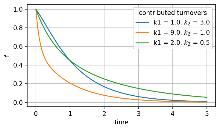
Turnover rates themselves can also be free parameters. Here cm2 uses a cascading two-state structure: state 0 loses molecules at rate k1 (no input from outside), and state 1 receives molecules from state 0 at rate k2 while clearing at the same rate. The rate matrix is:

M = [[-k1,  0 ],
     [ k2, -k2]]

Varying k1 and k2 changes both the shape of f(t) and the mean age of the population.

cm2 = SymbolicCompartmentalModel(n_states=2)

k1 = cm2.add_parameter(symbol="k1", lb=0.01, ub=10.0)
k2 = cm2.add_parameter(symbol="k2", lb=0.01, ub=10.0)
cm2.contributed_turnovers = [[-k1, 0.0], [k2, -k2]]
cm2.observed_pool_weights = [0.5, 0.5]
display("M = ", cm2.contributed_turnovers)

fig, ax = plt.subplots(1, 1, figsize=(5, 3), dpi=150)
for x_value in ([1.0, 3.0], [9.0, 1.0], [2.0, 0.5]):
    cm2.plot("f", x=x_value, ax=ax, label=f"k1 = {x_value[0]:.1f}, $k_2$ = {x_value[1]:.1f}",
             t_range=np.linspace(0.0, 5.0, 100))
ax.legend(title="contributed turnovers")
ax.grid(True)

fig.tight_layout()
if Path("../results").exists():
    fig.savefig("../results/example_2_state_2_parameters.svg")
display(fig)
plt.close(fig)

'M = '

Matrix([
[-k1,   0],
[ k2, -k2]])

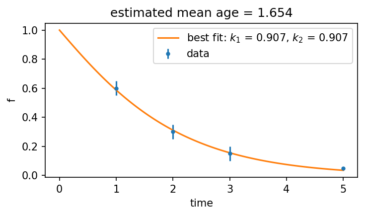
2.1.3. Fitting a CM to experimental data

tdata = np.array([1.0, 2.0, 3.0, 5.0])
ydata = np.array([0.6, 0.3, 0.15, 0.05])
ydata_err = np.array([0.05, 0.05, 0.05, 0.01])
fit_results = cm2.fit(tdata, ydata, check_mass_balance=False)

fig, ax = plt.subplots(1, 1, figsize=(5, 3), dpi=150)
ax.errorbar(tdata, ydata, yerr=ydata_err, fmt=".", label="data")
fit_results.cm.plot("f", x=[0.5, 4.0], ax=ax,
                    label=f"best fit: $k_1$ = {fit_results.popt[0]:.3f}, $k_2$ = {fit_results.popt[1]:.3f}",
                    t_range=np.linspace(0.0, 5.0, 100))
ax.legend()

best_fit_mean_age = fit_results.cm.mean_age()

ax.set_title(f"estimated mean age = {best_fit_mean_age:.3f}")
fig.tight_layout()
if Path("../results").exists():
    fig.savefig("../results/example_2_state_fitting.svg")
display(fig)
plt.close(fig)

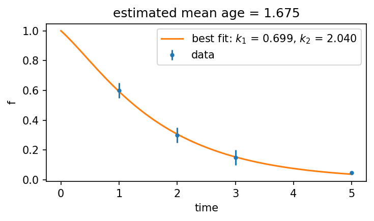
fit(tdata, ydata) minimizes the residual sum of squares between the model’s f(t) prediction and the observed labeling fractions. It returns a FitResult containing the best-fit parameter values (popt) and a ready-to-use model instance (fit_results.cm).

The mean age of the fitted model is a single summary statistic: it equals the area under the best-fit survival curve and represents the average time a molecule has spent in the system.

2.1.4. Applying the constraints imposed by mass-balance

This is the best fit given the data and the chosen model (2-state linear chain with equal pool weights). Now, if we want to assume that the pool weights are proportional to their sizes, then we can also introduce mass-balance constraints:

\[\mathbf{s}^\top (\mathbf{M} + \mu \mathbf{I}_n) \leq \mathbf{0}_n\]

Here, \(\mathbf{s} = (0.5, 0.5)\), and \(\mu = 0\), so if we plug in the \(\mathrm{M}\)-matrix and simplify the inequality, we get that the only constraint is \(k_1 > k_2\). As we can see, the best fit that we got does not qualify.

if fit_results.cm.is_mass_balanced():
    print("Fitted model is mass-balanced!")
else:
    print("Fitted model is not mass-balanced!")

Fitted model is not mass-balanced!

In order to comply with the mass-balance constraint, we can rerun the fit() while setting the relevant flag (check_mass_balance) to be True:

fit_results = cm2.fit(tdata, ydata, check_mass_balance=True)

fig, ax = plt.subplots(1, 1, figsize=(5, 3), dpi=150)
ax.errorbar(tdata, ydata, yerr=ydata_err, fmt=".", label="data")
fit_results.cm.plot("f", x=[0.5, 4.0], ax=ax,
                    label=f"best fit: $k_1$ = {fit_results.popt[0]:.3f}, $k_2$ = {fit_results.popt[1]:.3f}",
                    t_range=np.linspace(0.0, 5.0, 100))
ax.legend()

best_fit_mean_age = fit_results.cm.mean_age()

if fit_results.cm.is_mass_balanced():
    print("Fitted model is mass-balanced!")
else:
    print("Fitted model is not mass-balanced!")

ax.set_title(f"estimated mean age = {best_fit_mean_age:.3f}")
fig.tight_layout()
display(fig)
plt.close(fig)

Fitted model is mass-balanced!

So, now we can see that as expected \(k_1 \geq k_2\) (actually, they are equal) and that the mean age has barely changed. Moreover, the fitted curve is nearly identical to the previous one and fits the data just as well. This is a good example for the fact that, quite often, the turnover rates themselves have a wide range of solutions which all can fit the data very well. The mean age, however, is a more robust dynamic parameter.

2.1.5. Confidence calculations using a bootstrapping method

To quantify uncertainty in the mean-age estimate we use a bootstrap approach: draw N synthetic datasets by sampling from the measurement-noise distribution (a multivariate normal centred on the observed data), refit the model to each sample, and record the resulting mean ages. The empirical CDF of this distribution gives confidence intervals without requiring analytical error propagation.

N = 100
rng = np.random.default_rng(seed=2025)
y_samples = rng.multivariate_normal(
    mean=ydata,
    cov=np.diag(ydata_err),
    size=N,
)

mean_ages = []
k2_values = []
for i in tqdm(range(N)):
    y = y_samples[i, :]
    fit_results = cm2.fit(tdata, y)
    mean_ages.append(fit_results.cm.mean_age())
    k2_values.append(fit_results.popt[1])

fig, axs = plt.subplots(1, 2, figsize=(9, 4), dpi=120, sharey=True)
ax = axs[0]
ax.hist(mean_ages, cumulative=True, bins=1000, histtype='step', density=True)
ax.set_ylabel("Empirical cumulative distribution function (ECDF)")
ax.set_xlabel(r"Mean age ($\mathcal{{\bar{{A}}}}$)")
lb, ub = scipy.stats.scoreatpercentile(mean_ages, per=[25, 75])
ax.set_title(rf"$\mathcal{{\bar{{A}}}} \in$ ({lb:.1f}, {ub:.1f})");

ax = axs[1]
ax.hist(k2_values, cumulative=True, bins=1000, histtype='step', density=True)
ax.set_xlabel("2nd contributed turnover ($k_2$)")
lb, ub = scipy.stats.scoreatpercentile(k2_values, per=[25, 75])
ax.set_title(f"$k_2$ $\in$ ({lb:.1f}, {ub:.1f})");

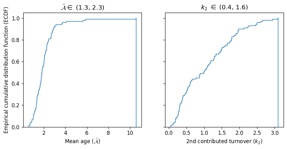
Comparing the two CDFs, one can see again that the mean age is a relatively more robust parameter (i.e., its distribution is more narrow).

Download notebook

Download this notebook