2.2. Examples for symbolic calculations with CM

A SymbolicCompartmentalModel can operate in two modes: numeric (returning float values) and symbolic (returning closed-form analytical expressions via SymPy). In symbolic mode, every model property is expressed as a formula in terms of the named parameters, which is useful for gaining analytical insight, deriving limiting cases, and understanding model behaviour across the full parameter space without running numerical simulations.

from symbolic_compartmental_model import SymbolicCompartmentalModel
import sympy
import matplotlib.pyplot as plt
from pathlib import Path

cm3 = SymbolicCompartmentalModel(n_states=2)
k1 = cm3.add_parameter(symbol="k1", lb=0.0, ub=10.0)
k2 = cm3.add_parameter(symbol="k2", lb=0.0, ub=10.0)
cm3.contributed_turnovers = [[-k1, 0.0], [0.0, -k2]]
cm3.observed_pool_weights = [0.5, 0.5]

We define a two-state CM where each state has an independent turnover rate (k1 and k2), and both contribute equally to the observed signal. Because the off-diagonal entries are zero the two states do not exchange molecules — the labeling curve is a symmetric bi-exponential 0.5·exp(−k1·t) + 0.5·exp(−k2·t).

print("\n\nmean age:")
display(sympy.simplify(cm3.as_symbolic("mean_age")))
print("\n\nmean residence time:")
display(sympy.simplify(cm3.as_symbolic("mean_residence_time")))
print("\n\nexpected decay rate:")
display(sympy.simplify(cm3.as_symbolic("expected_decay_rate")))
print("\n\nage CDF:")
display(sympy.simplify(cm3.as_symbolic("age_cdf")))
print("\n\nage PDF:")
display(sympy.simplify(cm3.as_symbolic("age_pdf")))
print("\n\nresidence time CDF:")
display(sympy.simplify(cm3.as_symbolic("residence_time_cdf")))
print("\n\nresidence time PDF:")
display(sympy.simplify(cm3.as_symbolic("residence_time_pdf")))
print("\n\ndecay rate:")
display(sympy.simplify(cm3.as_symbolic("decay_rate")))

mean age:

$\displaystyle \frac{0.5}{k_{2}} + \frac{0.5}{k_{1}}$

mean residence time:

$\displaystyle \frac{2.0}{k_{1} + k_{2}}$

expected decay rate:

$\displaystyle 0.5 k_{1} + 0.5 k_{2}$

age CDF:

$\displaystyle 1.0 - 0.5 e^{- k_{2} t} - 0.5 e^{- k_{1} t}$

age PDF:

$\displaystyle 0.5 k_{1} e^{- k_{1} t} + 0.5 k_{2} e^{- k_{2} t}$

residence time CDF:

$\displaystyle \frac{1.0 k_{1}}{k_{1} + k_{2}} - \frac{1.0 k_{1} e^{- k_{1} t}}{k_{1} + k_{2}} + \frac{1.0 k_{2}}{k_{1} + k_{2}} - \frac{1.0 k_{2} e^{- k_{2} t}}{k_{1} + k_{2}}$

residence time PDF:

$\displaystyle \frac{1.0 k_{1}^{2} e^{- k_{1} t}}{k_{1} + k_{2}} + \frac{1.0 k_{2}^{2} e^{- k_{2} t}}{k_{1} + k_{2}}$

decay rate:

$\displaystyle \frac{1.0 \left(k_{1}^{2} e^{k_{2} t} + k_{2}^{2} e^{k_{1} t}\right)}{k_{1} e^{k_{2} t} + k_{2} e^{k_{1} t}}$

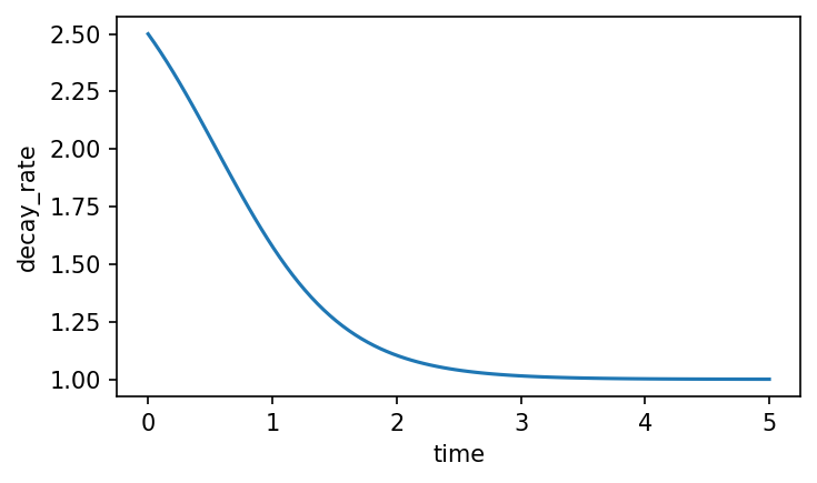
fig, ax = plt.subplots(1, 1, figsize=(5, 3), dpi=150)
cm3.plot("decay_rate", x=[1.0, 3.0], ax=ax)
fig.tight_layout()
if Path("../results").exists():
    fig.savefig("../results/decay_rate.svg")

as_symbolic(key) returns a SymPy expression for any of the following model properties:

Key	Meaning
mean_age	Expected age of a randomly chosen molecule (area under f(t))
mean_residence_time	Expected remaining lifetime from now (forward-looking)
expected_decay_rate	Instantaneous turnover rate averaged over the age distribution
age_cdf / age_pdf	Cumulative / probability density of molecular ages
residence_time_cdf / residence_time_pdf	Distribution of remaining lifetimes
decay_rate	Hazard function h(t) — instantaneous clearance rate given survival to age t

2.2.1. Growing system

cm3.growth_rate = 0.0
print("\n\nmean age:")
display(sympy.simplify(cm3.as_symbolic("mean_age")))
print("\n\nmean residence time:")
display(sympy.simplify(cm3.as_symbolic("mean_residence_time")))
cm3.growth_rate = 1.5
print("\n\nmean age:")
display(sympy.simplify(cm3.as_symbolic("mean_age")))
print("\n\nmean residence time:")
display(sympy.simplify(cm3.as_symbolic("mean_residence_time")))

mean age:

$\displaystyle \frac{0.5}{k_{2}} + \frac{0.5}{k_{1}}$

mean residence time:

$\displaystyle \frac{2.0}{k_{1} + k_{2}}$

mean age:

$\displaystyle \frac{0.5}{k_{2}} + \frac{0.5}{k_{1}}$

mean residence time:

$\displaystyle \frac{1.0 \left(k_{1} \left(1.0 k_{2} - 1.5\right) + k_{2} \left(1.0 k_{1} - 1.5\right)\right)}{\left(1.0 k_{1} - 1.5\right) \left(k_{1} + k_{2}\right) \left(1.0 k_{2} - 1.5\right)}$

The decay_rate (hazard function) h(t) describes how the probability of clearance changes as a molecule ages. For a single exponential h(t) is constant; for a multi-state model it varies with time, reflecting the shifting composition of the surviving population. At t = 0 the fast-clearing state dominates, driving a high initial hazard; as fast-clearing molecules are depleted the hazard decreases toward the rate of the slower state.

In a growing cell population, cell division continuously dilutes all molecules, adding an apparent clearance term μ to every state. Setting growth_rate = μ incorporates this into the model.

This affects ``mean_residence_time`` (forward-looking — accounts for future dilution by growth) but not ``mean_age`` (retrospective — describes molecules that already exist). Setting growth_rate = 0 recovers the non-growing case.

Download notebook

Download this notebook