2.3. Advanced code examples
This notebook covers three advanced topics:
Model validation and mass balance — checking that a CM is physically consistent before using it.
Multi-pool fitting — simultaneously fitting labeling data from multiple distinct observable pools to a single shared CM.
Model selection with BIC — using the Bayesian Information Criterion to choose the appropriate number of states without overfitting.
2.3.1. Model validation and mass-balance
[1]:
from symbolic_compartmental_model import SymbolicCompartmentalModel
import numpy as np
import matplotlib.pyplot as plt
import seaborn as sns
from pathlib import Path

sns.set_style("whitegrid")

# Create an invalid model that violates mass balance
cm = SymbolicCompartmentalModel(n_states=2)
cm.contributed_turnovers = [[-1, 2], [2, -2]]
cm.observed_pool_weights = [0.9, 0.1]
cm.growth_rate = 3.0

# Check if the model is valid (it is not because the sum of the first row is positive)
if cm.is_valid(raise_exception=False):
    print("Model is valid!")
else:
    print("Model is invalid!")
    print("row sums = ", np.sum(cm.M(), axis=1), " should all be non-positive\n\n")

# Fix the model validity
cm.contributed_turnovers = [[-1, 0], [2, -2]]

# Check again if the model is valid (now it should be)
if cm.is_valid(raise_exception=False):
    print("Model is valid!")
    print("row sums = ", np.sum(cm.M(), axis=1), " are all non-positive\n\n")
else:
    print("Model is invalid!")

# Check that the model is M-mass balanced (it is not)
if cm.is_M_mass_balanced(raise_exception=False):
    print("Model is M-mass balanced!")
else:
    print("Model is not M-mass balanced!")
    print("abscissa = ", cm.abscissa(), " should be smaller or equal to -μ = ", -cm.growth_rate, "\n\n")
cm.growth_rate = 1.0

# Check that the model is M-mass balanced (now it is)
if cm.is_M_mass_balanced(raise_exception=False):
    print("Model is M-mass balanced!")
    print("abscissa = ", cm.abscissa(), " is smaller or equal to -μ = ", -cm.growth_rate, "\n\n")
else:
    print("Model is not M-mass balanced!")


# Check if the model is mass-balanced
if cm.is_mass_balanced(raise_exception=False):
    print("Model is mass balanced!")
else:
    print("Model is not mass balanced!")
    print("s'(M + Iμ) = ", cm.s().T @ cm._M_plus_mu_I(), " should all be non-positive\n\n")

# Fix the model mass-balancing
cm.growth_rate = 0.7

# Check again if the model is mass-balanced
if cm.is_mass_balanced(raise_exception=False):
    print("Model is mass balanced!")
    print("s'(M + Iμ) = ", cm.s().T @ cm._M_plus_mu_I(), " are all non-positive\n\n")
else:
    print("Model is not mass balanced!")
Model is invalid!
row sums =  [1. 0.]  should all be non-positive


Model is valid!
row sums =  [-1.  0.]  are all non-positive


Model is not M-mass balanced!
abscissa =  -1.0  should be smaller or equal to -μ =  -3.0


Model is M-mass balanced!
abscissa =  -1.0  is smaller or equal to -μ =  -1.0


Model is not mass balanced!
s'(M + Iμ) =  [[ 0.2 -0.1]]  should all be non-positive


Model is mass balanced!
s'(M + Iμ) =  [[-0.07 -0.13]]  are all non-positive
A physically meaningful CM must satisfy 3 conditions:
Validity: the contributed_turnovers (\(\mathbf{M}\)-matrix) must obey the condition that all rows have a non-positive sum (i.e., the diagonal value, which is negative, must be larger in absolute value than the sum of all the other values in the row).
Mass balance: at steady-state the total efflux from the each state must larger or equal to the dilution by growth. Formally, the condition can be written as:
where \(\mathbf{s}\) are the observed_pool_weights, \(\mu\) is the growth rate, \(\mathbf{I}_n\) is the identity matrix of size \(n\), and \(\mathbf{0}_n\) is a vector of zeros.
M-mass balance: for a CM to be M-mass balanced, the M-matrix must satisfy the condition that the abscissa (the largest eigenvalue, which is a negative number) must be smaller or equal to \(-\mu\). This condition is necessary and sufficient for the existence of an assignment for \(\mathbf{s}\) that satifies the mass balance condition.
2.3.2. Fitting multiple pool data to a multi-state CM
[2]:
# Create a more complex model with parameters
cm_multi = SymbolicCompartmentalModel(n_states=3)

k1 = cm_multi.add_parameter(symbol="k1", lb=0.1, ub=5.0)
k2 = cm_multi.add_parameter(symbol="k2", lb=0.1, ub=10.0)
k3 = cm_multi.add_parameter(symbol="k3", lb=0.1, ub=2.0)

cm_multi.contributed_turnovers = [[-k1, 0, 0], [k1, -k2, 0], [0, k2, -k3]]
cm_multi.observed_pool_weights = [0.2, 0.3, 0.5]

# Multi-pool experimental data: (pool_id, time, measurement)
multi_pool_data = [
   (0, 1.0, 0.8), (0, 2.0, 0.6), (0, 3.0, 0.4),
   (1, 1.0, 0.9), (1, 2.0, 0.7), (1, 3.0, 0.5),
   (2, 1.0, 0.95), (2, 2.0, 0.85), (2, 3.0, 0.7)
]

# Fit with mass balance constraint
fit_results = cm_multi.fit_multiple_pools(multi_pool_data)
print(fit_results)
print(f"RSS: {fit_results.rss:.6f}")
print(f"Mean ages: {fit_results.cm.mean_ages()}")

fig, ax = plt.subplots(1, 1, figsize=(4, 4), dpi=150)

colors = ["cyan", "orange", "green"]
for idx, t, y in multi_pool_data:
    fit_results.cm.observed_pool_weights = np.eye(3)[idx,:]
    fit_results.cm.plot(key="f", ax=ax, color=colors[idx], alpha=0.2)
    ax.plot(t, y, 'x', color=colors[idx])
ax.set_xlabel("time, t")
ax.set_ylabel("labeling, f(t)")
if Path("../results").exists():
    fig.savefig("../results/example_multiple_pools.svg")
Best fit parameters: k1 = 0.2788, k2 = 0.4448, k3 = 0.4912
n_samples = 9, RSS = 0.01177, ΔAIC = -53.76, BIC = -53.17
RSS: 0.011766
Mean ages: [3.58730091 4.49612418 6.1073787 ]
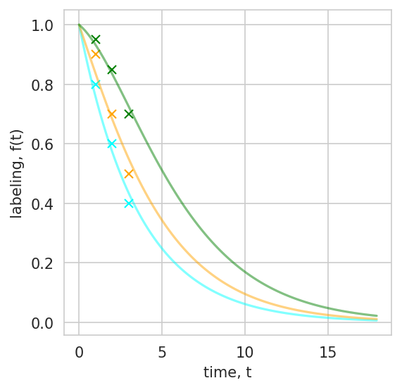
When labeling data is available for multiple observable pools (e.g. different cellular fractions, subunits, or protein complexes), all measurements can be fit simultaneously to a single shared CM. Each data point is a triplet (pool_id, time, measurement), where pool_id selects which linear combination of internal states defines the observable for that measurement.
fit_multiple_pools() optimizes the shared kinetic parameters to minimize the total residual across all pools, ensuring one mechanistic model is consistent with every observation. The returned FitResult also exposes mean_ages() — the per-state mean age vector — in addition to the scalar mean age of the observed mixture.
2.3.3. Using BIC to choose between different models
[3]:
# Generate synthetic data with noise
cm_ground_truth = SymbolicCompartmentalModel(n_states=2)
cm_ground_truth.contributed_turnovers = [[-1.0, 0], [0.5, -0.5]]
cm_ground_truth.observed_pool_weights = [0.2, 0.8]

np.random.seed(42)
t_data = np.array([0.1, 0.2, 0.3, 0.5, 1.0, 1.5, 2.0, 3.0, 4.0])
y_true = cm_ground_truth.f()(t_data)
y_data = y_true + 0.02 * np.random.randn(len(y_true))  # Add noise

# Try to fit a single pool CM to the data
cm_one = SymbolicCompartmentalModel(n_states=1)
k = cm_one.add_parameter(symbol="k", lb=0.1, ub=10.0)
cm_one.contributed_turnovers = [[-k]]

# Add parameters with different constraints
cm_two = SymbolicCompartmentalModel(n_states=2)
k1 = cm_two.add_parameter(symbol="k1", lb=0.1, ub=10.0)
k2 = cm_two.add_parameter(symbol="k2", lb=0.1, ub=10.0)
w = cm_two.add_parameter(symbol="w", lb=0, ub=1)
cm_two.contributed_turnovers = [[-k1, 0.0], [k2, -k2]]
cm_two.observed_pool_weights = [w, 1-w]

# Use minimize instead of curve_fit for better control
fit_results_one = cm_one.fit(
    tdata=t_data,
    ydata=y_data,
)
# Use minimize instead of curve_fit for better control
fit_results_two = cm_two.fit(
    tdata=t_data,
    ydata=y_data,
)

print("1-state model\n", fit_results_one)
print("\n\n2-state model\n", fit_results_two)

fig, ax = plt.subplots(1, 1, figsize=(4, 4), dpi=150)
fit_results_one.cm.plot(key="f", ax=ax, t_range=np.linspace(0, 4, 100), color="red", label="1-state")
fit_results_two.cm.plot(key="f", ax=ax, t_range=np.linspace(0, 4, 100), color="green", label="2-state")
ax.plot(t_data, y_true, 'x', label="experimental data", color="blue")
ax.legend()
ax.set_xlabel("time, t")
ax.set_ylabel("labeling, f(t)")
if Path("../results").exists():
    fig.savefig("../results/example_bic.svg")
1-state model
 Best fit parameters: k = 0.333
n_samples = 9, RSS = 0.01362, ΔAIC = -56.44, BIC = -56.25


2-state model
 Best fit parameters: k1 = 0.9503, k2 = 0.5227, w = 0.1781
n_samples = 9, RSS = 0.001844, ΔAIC = -70.44, BIC = -69.85
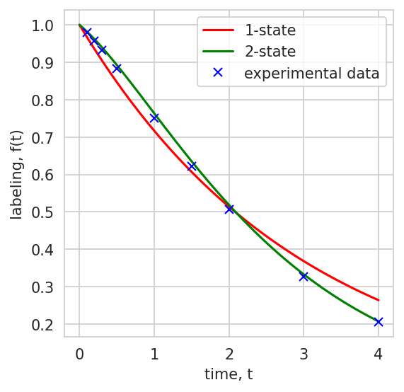
A more complex model always fits the training data better, but may overfit noise. For the Gaussian special case, the Bayesian Information Criterion (BIC) is defined as:
where \(n\) is the number of free parameters, \(m\) is the number of observed data points, and \(\text{RSS}\) is the residual sum of squares between the fitted curve and the data points. A lower BIC indicates a better trade-off between fit quality and parsimony.
Download notebook